TRIXについて、計算式、チャート、エクセルVBAコード。

 

TRIXは終値の自然対数を指数移動平均（EMA）で3回平均化した数値と前日との差から求められる指標です。

 

 

 

TRIXの計算式（Nは足数）

 

EMA1 = N(close)のN本指数平滑移動平均

※N(close)=終値の自然対数

EMA2 = EMA1のN本指数平滑移動平均

EMA3 = EMA2のN本指数平滑移動平均

TRIX = (EMA3 – 前日のEMA3) × 10000

 

指数平滑移動平均線⇒ https://atmtech.net/main/?p=2890

 

 

TRIXのチャート

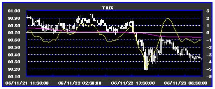
(黄色線TRIX5　赤線TRIX30)

 

 

TRIXのVBAコード

‘※　エクセルの1列目(A列)に行番号、2列目(B列)に日時、
‘※　3列目(C列)～6列目(F列)に始値・高値・安値・終値
‘********************************
‘ n ：TRIXの採用本数
‘ num：現在の行
‘ r_now：現在値
‘ cell_ln：終値自然対数書込み列
‘ cell_ema1：指数平滑線1計算値書込み列
‘ cell_ema2：指数平滑線1計算値書込み列
‘ cell_ema3：指数平滑線1計算値書込み列
‘ cell_trix：指数平滑線1計算値書込み列
‘********************************
‘*******自然対数
If Cells(num, 6) <> “” Then
Cells(num, cell_ln) = Application.Ln(Cells(num, 6))
End If
‘*******EMA1
If num – 2 = n Then
Cells(num, cell_ema1) = Application.WorksheetFunction.Average _
(.Range(Cells(num – (n – 1), cell_ln), Cells(num, cell_ln)))
End If
If num – 2 > n Then
Cells(num, cell_ema1) = Cells(num – 1, cell_ema1) + _
((Cells(num, cell_ln) – Cells(num – 1, cell_ema1)) * 2 / (1 + n))
End If
‘*******EMA2
If num – 2 = n + (n – 1) Then
Cells(num, cell_ema2) = Application.WorksheetFunction.Average _
(.Range(Cells(num – (n – 1), cell_ema1), Cells(num, cell_ema1)))
End If
If num – 2 > n + (n – 1) Then
Cells(num, cell_ema2) = Cells(num – 1, cell_ema2) + _
((Cells(num, cell_ema1) – Cells(num – 1, cell_ema2)) * 2 / (1 + n))
End If
‘*******EMA3
If num – 2 = 2 * n + (n – 2) Then
Cells(num, cell_ema3) = Application.WorksheetFunction.Average _
(.Range(Cells(num – (n – 1), cell_ema2), Cells(num, cell_ema2)))
End If
If num – 2 > 2 * n + (n – 2) Then
Cells(num, cell_ema3) = Cells(num – 1, cell_ema3) + _
((Cells(num, cell_ema2) – Cells(num – 1, cell_ema3)) * 2 / (1 + n))
End If
‘*******TRIX
If Cells(num – 1, cell_ema3) <> “” Then
Cells(num, cell_trix) = (Cells(num, cell_ema3) – _
Cells(num – 1, cell_ema3)) * 10000
End If

 

 

テクニカル指標一覧

罫線談義一覧

(外部リンク)テクニカル指標(Wikipedia)